User Guide

This manual is intended to help you get started with PLASMAG. Most of the features are described exhaustively.

Installation

We recommend to use a Python virtual environment to run PLASMAG. In the following explanation, we will use Conda [1] to prepare the environment. If you don’t have it already, please refer to this page to install it: https://conda.io/projects/conda/en/latest/user-guide/install/index.html

Getting PLASMAG

PLASMAG’s repository is reachable at: https://github.com/LaboratoryOfPlasmaPhysics/PLASMAG

To use it you can either download a tagged version or clone the most recent state of the master branch.

Installing prerequisites

Open a terminal (or an Anaconda PowerShell prompt under Windows)
Go to the main folder of PLASMAG
Execute the following command to create a virtual environment with all needed prerequisites:

conda env create -f user_environment.yml

Activate the environment

conda activate PLASMAG

[Windows only] If you’re running Windows, you need to copy manually a library where Python will search for it. For that the first step is to identify the path of your virtual environment:
```
where python
```
Let’s name <path_of_your_environment> the answer, to which you remove “python.exe”. Then copy the file “ngspice.dll” from <path_of_your_environment>/bin/ to <path_of_your_environment>/lib/Site_packages/PySpice/Spice/NgSpice/Spice64_dll/dll-vs/ (the two last folders has to by created before)
Run the application

python PLASMAG.py

Whenever you open a new terminal (or an Anaconda PowerShell prompt), you will need to do the activation (conda activate PLASMAG) step before running the application.

Footnotes

Global presentation of the User Interface

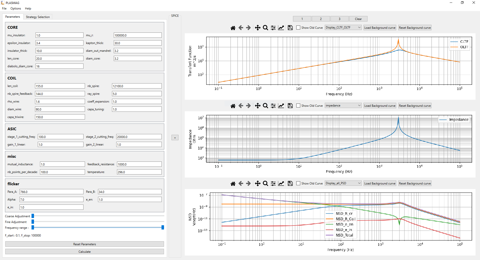
The UI is divided into three main sections: the menubar, the parameter panel, and the canvas.

Menubar

The menubar is located at the top of the window and contains the following menus:

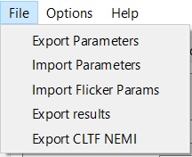
File: this menu gives access to import and export features (see the Feature section below for more details)
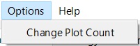
Options: this menu gives access to the parametrisation of the number of plots in the Canva area
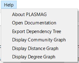
Help: this menu gives access to the documentation and to some representation of the way the different physical quantities are related (nodes dependencies)

Tabs

It’s used to switch between different functionalities of the program.

Parameters Section

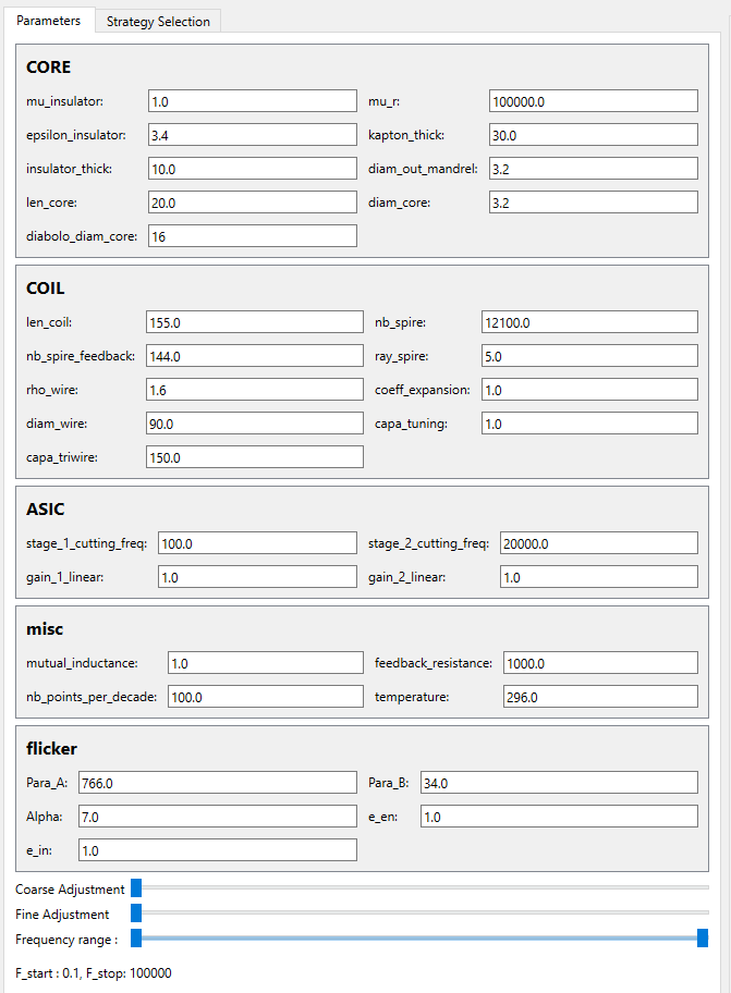
The parameters section is located on the left side of the window and contains the parameters of the simulation. All of the parameters are grouped by category.

How to change a parameter

Option 1:

Click on the line edit field of the parameter you want to change
Enter the new value
Press Enter
If the value is valid, the calculation will be triggered. If the value is invalid, the field will turn red and the calculation will not be triggered.

Option 2:

Click on the line edit field of the parameter you want to change
Use the sliders to change the value, the value will be updated in real time and the calculation will be triggered

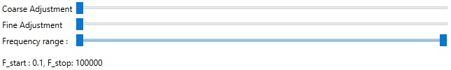
At every moment, you can reset the value of a parameter by clicking on the reset button. Or force trigger the calculation by clicking on the calculate button. You can use the frequency range double slider to select the frequency range you want to simulate.

Strategy selection

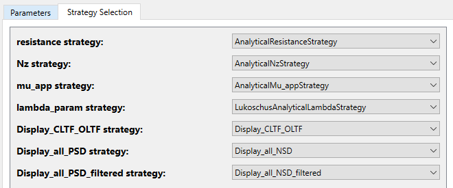
One of the most importants features of PLASMAG is to be modular and to allow the user to choose the strategy he wants to use to simulate a particular value (like the resistance, the capacitance, etc…). You can easily implement your own strategy by following the instructions in the Contributing new code section. If you did everything well, your strategy will appear in the strategy selection combobox. You can now select it and it will be used in the simulation.

When you select a strategy if an error occurs, the error message will be displayed in a popup. It often means that the parameters are not valid for the selected strategy, or your implementation is not valid and implicate cyclic dependencies between differents calculations nodes.

Canvas

The canvas is located on the right side of the window and contains the plots of the simulation. You can adjust the number of plots displayed by clicking on the options button and changing the plot count (from 1 to 5, default 3)

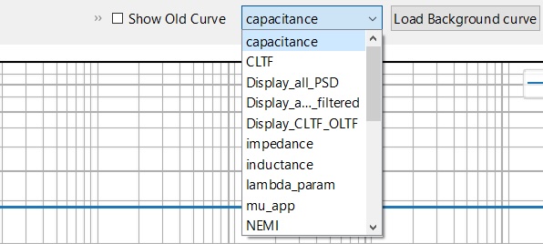
Using the combo box you can chose to display whatever you want in the plot. The list contains every node that can be calculated in the program. The graph will be updated in real time when you change the parameters. The data is linear but plotted in a logarithmic scale, for x and y axis.

If you want to fit existing data by tuning parameters, you can load a curve in background by clicking on the load curve button. You can then select a csv file that contains the curve you want to display. The file must be composed of 2 columns (frequencies and values) separated by commas, and the frequency must be in Hz.

Memory

As PLASMAG is a tuning tool, it’s important to be able to compare the results of different simulations. To do so, you can save the results of a simulation by clicking on one of the save button (1,2,3). The results/parameters will be saved in memory and you can load them back by clicking on the load button.
When data are stored in memory, the save button will turn green.
You can “reset” parameters to the saved state by clicking again on a green save button.
Memory is not saved when you close the program (please use the Export Parameters feature for a more permanent saving).
You can clear the memory by clicking on the clear memory button.

Features

Analytical model

Resistance (R) Node

The resistance node proposes 2 analytical strategies:

class src.model.strategies.strategy_lib.resistance.AnalyticalResistanceStrategy

Analytical model of the resistance of a monolayer winding

\[R = N_{spire} . 2 . \pi . R_s . \rho_{wire}\]

with:

\(N_{spire}\) : number of spire of the coil
\(R_s\) : radius of the spires
\(\rho_{wire}\) : linear resistance of the wire

class src.model.strategies.strategy_lib.resistance.MultiLayerResistanceStrategy

Analytical model of the resistance of a multi-layer winding

\[R = \rho_{wire} . (l_{main\_coil} + l_{feedback})\]

with:

\(\rho_{wire}\) : linear resistance of the wire

\(l_{main\_coil}\) being the length of the main coil, computed with:

\(l_{main\_coil} = \pi . Ns_{per\_layer\_mc} . N_{layers} . (d_{out\_mandrel} + N_{layers} . d_{wire} + (N_{layers} - 1) . K_t)\)

\(Ns_{per\_layer\_mc}\) : the number of spires on each of the main coil layers

\(N_{layers}\) : the number of coil layers

\(d_{out\_mandrel}\) : the output diameter of the mandrel

\(d_{wire}\) : the diameter of the wire

\(K_t\) : the Kapton thick

\(l_{feedback}\) being the length of the feedback coil, computed with:

\(l_{feedback} = \pi . Ns_{per\_layer\_fb} . N_{layers} . (d_{out\_mandrel} + (N_{layers} + 1) . d_{wire} + (N_{layers} - 1) . K_t)\)

\(Ns_{per\_layer\_fb}\) : the number of spires on each of the feedback coil layers

Magnetometric demagnetizing factor (\(N_z\)) Node

The magnetometric demagnetizing factor node proposes 2 analytical strategies:

class src.model.strategies.strategy_lib.Nz.AnalyticalNzStrategy

Magnetometric demagnetizing coefficient in the core axis direction for a cylindrical core shape

\[N_z = \frac{d_{core}}{2 . l_{core} + d_{core}}\]

with:

\(d_{core}\) : the diameter of the core
\(l_{core}\) : the length of the core

class src.model.strategies.strategy_lib.Nz.AnalyticalNzDiaboloStrategy

Magnetometric demagnetizing coefficient in the core axis direction for a diabolo core shape

\[N_z = \frac{\ln(2.m) - 1}{m^2}\]

with:

\(m = l_{core} / d_{diabolo}\)
\(l_{core}\) : the length of the core (including diabolo shape)
\(d_{diabolo}\) : the diameter of the end surface of the diabolo

Effective permeability (\(\mu_{app}\)) Node

The effective permeability node proposes 2 analytical strategies:

class src.model.strategies.strategy_lib.mu_app.AnalyticalMu_appStrategy

Analytical model of the effective permeability for a cylindrical core

\[\mu_{app} = \frac{\mu_r}{1 + (N_z . (\mu_r - 1))}\]

with:

\(\mu_r\) : the relative permeability of the core material
\(N_z\) : the demagnetizing factor, related to the shape of the material

class src.model.strategies.strategy_lib.mu_app.AnalyticalMu_appDiaboloStrategy

Analytical model of the effective permeability for a diabolo core

\[\mu_{app} = \frac{\mu_r}{1 + (N_z . \frac{d_{core}^2}{d_{diabolo}^2} . (\mu_r - 1))}\]

with:

\(\mu_r\) : the relative permeability of the core material
\(N_z\) : the demagnetizing factor, related to the shape of the material
\(d_{core}\) : the diameter of the center of the core
\(d_{diabolo}\) : the diameter of the end surface of the diabolo

Lambda coefficient factor (\(\lambda\)) Node

The lambda coefficient factor node proposes 2 analytical strategies:

class src.model.strategies.strategy_lib.lambda_strategy.LukoschusAnalyticalLambdaStrategy

Lukoschus’s analytical computation of the coefficient factor

\[\lambda = (\frac{l_{coil}}{l_{core}})^\frac{-2}{5}\]

with:

\(l_{coil}\) : the length of the coil
\(l_{core}\) : the length of the core

class src.model.strategies.strategy_lib.lambda_strategy.ClercAnalyticalLambdaStrategy

Clerc’s analytical computation of the coefficient factor

\[\lambda = 1.85 - 1.1 * \frac{l_{coil}}{l_{core}}\]

with:

\(l_{coil}\) : the length of the coil
\(l_{core}\) : the length of the core

Inductance (L) Node

The inductance is computed as follow:

class src.model.strategies.strategy_lib.inductance.AnalyticalInductanceStrategy

Analytical model of the inductance

\[L = \mu_0 . \mu_{app} . N_{spire}^2 . S . \lambda_{param} / l_{core}\]

with:

\(\mu_0\) : permeability of vacuum
\(\mu_{app}\) : apparent permeability of the core material
\(N_{spire}\) : number of spire of the coil
\(S = \pi . R_s^2\) le section of the core
\(R_s\) : radius of the spires
\(\lambda_{param}\) : coefficient factor (see lambda node for more information)
\(l_{core}\) : the length of the core

Capacitance (C) Node

The capacitance is computed as follow:

class src.model.strategies.strategy_lib.capacitance.AnalyticalCapacitanceStrategy

Analytical model of the capacitance

\[C = \frac{\pi . \epsilon_0 . \epsilon_{insulator} . l_{coil}}{(K_t + 2 * I_t) . N_{layer}^2} . (N_{layer} - 1) . (d_{out\_mandrel} + N_{layer} . d_{wire} + (N_{layer} - 1) . K_t) + C_{tuning} + C_{triwire}\]

with:

\(\epsilon_0\) : vacuum permittivity
\(\epsilon_{insulator}\) : the permittivity of the insulator
\(l_{coil}\) : the length of the coil
\(K_t\) : Kapton thick
\(I_t\) : Insulator thick
\(N_{layer}\) : number of coil layers
\(d_{out\_mandrel}\) : the output diameter of the mandrel
\(d_{wire}\) : the diameter of the wire
\(C_{tuning}\) : tuning capacitance
\(C_{triwire}\) : triwire capacitance

Impedance (Z) Node

The impedance is computed as follow:

class src.model.strategies.strategy_lib.impedance.AnalyticalImpedanceStrategy

Analytical model of the impedance

\[Z(f) = \sqrt{\frac{R^2 + \omega^2}{(1 - L . C . \omega^2)^2 + (\omega . R . C)^2}}\]

with:

\(R\) : resistance of the coil
\(L\) : inductance of the coil
\(C\) : capacitance of the coil
\(\omega = 2 \pi f\)
\(f\) : frequency

ASIC’s transfer function (\(H\), \(H_1\) and \(H_2\)) Nodes

The ASIC transfer function is the product of both stage’s transfer function. Here are the strategies for each stage and for the whole ASIC.

class src.model.strategies.strategy_lib.TF_ASIC.TF_ASIC_Stage_1_Strategy_linear

Analytical model for ASIC stage 1 transfer function

\[H_1(f) = \frac{gain_1}{\sqrt{1 + (\frac{f}{f_{c1}})^2}}\]

with:

\(gain_1\) : gain of the ASIC’s stage 1
\(f\) : the frequency
\(f_{c1}\) : the cutting frequency of the 1st stage of the ASIC

class src.model.strategies.strategy_lib.TF_ASIC.TF_ASIC_Stage_2_Strategy_linear

Analytical model for ASIC stage 2 transfer function

\[H_2(f) = \frac{gain_2}{\sqrt{1 + (\frac{f}{f_{c2}})^2}}\]

with:

\(gain_2\) : gain of the ASIC’s stage 2
\(f\) : the frequency
\(f_{c2}\) : the cutting frequency of the 2nd stage of the ASIC

class src.model.strategies.strategy_lib.TF_ASIC.TF_ASIC_Strategy_linear

Analytical model of the total ASIC transfer function

\[H(f) = H_1(f) . H_2(f)\]

with:

\(H_1\) : transfer function of the ASIC’s stage 1
\(H_2\) : transfer function of the ASIC’s stage 2
\(f\) : the frequency

Open Loop Transfer Function (OLTF)

This strategy returns 2 transfer functions: the first one “OLTF” is not impacted by the ASIC’s 2nd stage, the second “OLTF_filtered” is filtered by the ASIC’s 2nd stage. Both are plotted together on the “OLTF” plot.

class src.model.strategies.strategy_lib.OLTF.OLTF_Strategy

Analytical model of the Open Loop Transfer Function (OLTF)

\[OLTF(f) = \frac{\mu_{app} . N_s . S . \omega . H_1(f)}{\sqrt{(1 - L . C . \omega^2)^2 + (\omega . R . C)^2}}\]

With:

\(\mu_{app}\) : apparent permeability of the core material
\(N_{spire}\) : number of spire of the coil
\(S = \pi . R_s^2\) le section of the core
\(R_s\) : radius of the spires
\(\omega = 2 \pi f\)
\(f\) : frequency
\(H_1\) : transfer function of the ASIC’s stage 1
\(R\) : resistance of the coil
\(L\) : inductance of the coil
\(C\) : capacitance of the coil

Closed Loop Transfer Function (CLTF)

This strategy returns 2 transfer functions: the first one “CLTF” is not impacted by the ASIC’s 2nd stage, the second “CLTF_filtered” is filtered by the ASIC’s 2nd stage. Both are plotted together on the “CLTF” plot.

class src.model.strategies.strategy_lib.CLTF.CLTF_Strategy

Analytical model of the Closed Loop Transfer Function (CLTF)

\[CLTF(f) = \frac{\mu_{app} . N_s . S . \omega . H_1(f)}{\sqrt{(1 - L . C . \omega^2)^2 + \omega^2 . (R . C + \frac{M . H_1(f)}{R_{CR}})^2}}\]

With:

\(\mu_{app}\) : apparent permeability of the core material
\(N_{spire}\) : number of spire of the coil
\(S = \pi . R_s^2\) le section of the core
\(R_s\) : radius of the spires
\(\omega = 2 \pi f\)
\(f\) : frequency
\(H_1\) : transfer function of the ASIC’s stage 1
\(R\) : resistance of the coil
\(L\) : inductance of the coil
\(C\) : capacitance of the coil
\(M\) : Mutual inductance (coupling factor between the main coil and the feedback coil)
\(R_{CR}\) : resistance of the counter-reaction coil

Noises Spectral Densities

The spectral densities here are all computed in \(\frac{V}{\sqrt{Hz}}\) and called Noise Spectral Densities. They are plotted together in the “Display_all_PSD” plot (still as Noise Spectral Densities)

They can be rendered in \(\frac{V^2}{Hz}\) (real Power Spectral Density) by using “Display_all_PSD_strategy” in the Strategy Selection tab.

Except for the Flicker noise spectral density, all the spectral density strategies return 2 quantities: the first one “NSD_XX” is not impacted by the ASIC’s 2nd stage, the second “NSD_XX_filtered” is filtered by the ASIC’s 2nd stage. Both are plotted together on the “NSD_XX” plot.

The “NSD_filtered_Total” is the quadratic sum of the filtered NSD_XX.

All the filtered spectral densities are plotted together on the “Display_all_PSD_filtered” while all the non-filtered are plotted together on the “Display_all_PSD”

class src.model.strategies.strategy_lib.Noise.NSD_R_cr

Analytical model for counter-reaction resistance (\(R_{CR}\)) Noise Spectral Density

\[NSD_{R_{CR}}(f) = \sqrt{\frac{|4 . k . T . R_{CR}| . \omega^2 . (\frac{M . H_1}{R_{CR}})^2}{(1 - L . C . \omega^2)^2 + \omega^2 . (R . C + \frac{M . H_1}{R_{CR}})^2}}\]

With:

\(k\) : the Boltzmann constant
\(T\) : the temperature
\(R_{CR}\) : resistance of the counter-reaction coil
\(\omega = 2 \pi f\)
\(f\) : frequency
\(M\) : Mutual inductance (coupling factor between the main coil and the feedback coil)
\(H_1\) : transfer function of the ASIC’s stage 1
\(R\) : resistance of the coil
\(L\) : inductance of the coil
\(C\) : capacitance of the coil

class src.model.strategies.strategy_lib.Noise.NSD_R_Coil

Analytical model for coil resistance (\(R_{Coil}\)) Noise Spectral Density

\[NSD_{R_{Coil}}(f) = \sqrt{\frac{|4 . k . T . R|}{(1 - L . C . \omega^2)^2 + \omega^2 . (R . C + \frac{M . H_1}{R_{CR}})^2}}\]

With:

\(k\) : the Boltzmann constant
\(T\) : the temperature
\(R\) : resistance of the coil
\(\omega = 2 \pi f\)
\(f\) : frequency
\(M\) : Mutual inductance (coupling factor between the main coil and the feedback coil)
\(H_1\) : transfer function of the ASIC’s stage 1
\(L\) : inductance of the coil
\(C\) : capacitance of the coil

class src.model.strategies.strategy_lib.Noise.NSD_Flicker

Analytical model for flicker noise (\(NSD_{Flicker}\)) Noise Spectral Density

\[NSD_{flicker}(f) = \frac{Para_A . 10^{-9}}{Para_B . f^\frac{\alpha}{10}} + e_{en}\]

with:

\(Para_A\) : fitting parameter adjusting the amplitude of the noise curve
\(Para_B\) : fitting parameter adjusting the noise’s frequency dependency
\(f\) : frequency
\(\alpha\) : exponent parameter fine-tuning the frequency scaling
\(e_{en}\) : equivalent input noise voltage

class src.model.strategies.strategy_lib.Noise.NSD_e_en

Analytical model for equivalent input noise voltage (\(e_en\)) Noise Spectral Density

\[NSD_{e_{en}}(f) = \sqrt{\frac{H_1^2(f) . NSD_{flicker}^2(f) . (1 - L . C . \omega^2)^2 + (\omega . R . C)^2}{(1 - L . C . \omega^2)^2 + \omega^2 . (R . C + \frac{M . H_1(f)}{R_{CR}})^2}}\]

With:

\(H_1\) : transfer function of the ASIC’s stage 1
\(NSD_{flicker}\) : Noise Spectral Density of flicker noise
\(L\) : inductance of the coil
\(C\) : capacitance of the coil
\(\omega = 2 \pi f\)
\(f\) : frequency
\(R\) : resistance of the coil
\(M\) : Mutual inductance (coupling factor between the main coil and the feedback coil)
\(R_{CR}\) : resistance of the counter-reaction coil

class src.model.strategies.strategy_lib.Noise.NSD_e_in

Analytical model for input noise current (\(e_in\)) Noise Spectral Density

\[NSD_{e_{in}}(f) = \sqrt{\frac{Z^2(f) . (e_{in} . 10^{-3})^2 . H_1^2(f) . (1 - L . C . \omega^2)^2 + (\omega . R . C)^2}{(1 - L . C . \omega^2)^2 + \omega^2 . (R . C + \frac{M . H_1(f)}{R_{CR}})^2}}\]

With:

\(Z\) : Impedance
\(e_{in}\) : the input noise current level
\(H_1\) : transfer function of the ASIC’s stage 1
\(L\) : inductance of the coil
\(C\) : capacitance of the coil
\(\omega = 2 \pi f\)
\(f\) : frequency
\(R\) : resistance of the coil
\(M\) : Mutual inductance (coupling factor between the main coil and the feedback coil)
\(R_{CR}\) : resistance of the counter-reaction coil

class src.model.strategies.strategy_lib.Noise.NSD_Total

Analytical model for total Noise Spectral Density

\[NSD_{total}(f) = \sqrt{NSD_{e_{in}}^2(f) + NSD_{e_{en}}^2(f) + NSD_{R_{Coil}}^2(f) + NSD_{R_{CR}}^2(f)}\]

With:

\(NSD_{e_{in}}\) : input noise current (\(e_in\)) Noise Spectral Density
\(NSD_{e_{en}}\) : equivalent input noise voltage (\(e_en\)) Noise Spectral Density
\(NSD_{R_{Coil}}\) : coil resistance (\(R_{Coil}\)) Noise Spectral Density
\(NSD_{R_{CR}}\) : counter-reaction resistance (\(R_{CR}\)) Noise Spectral Density

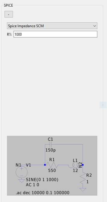
SPICE

Parameters export and import

Through the File menu in the menubar, you can export or import parameters and data.

The JSON format has been chosen to allow both user and computer to read and write the parameters files easily. The available features are:

Export Parameters: exports the whole set of current parameters of to a JSON file.

Import Parameters: imports the parameters from a JSON file (same structure as exported files). If some parameters are missing from your file, they will be taken in default.json
Import Flicker Params: imports the flicker parameters from a JSON file formatted like this:
{
    "Para_A": 615.0,
    "Para_B": 34.0,
    "Alpha": 7.0,
    "e_en": 3.0,
    "e_in": 106.0
}
Be careful that your values are inside the limits defined by the last file loaded through Import Parameters or those defined in default.json.
Export Results: exports the results of the simulation to a CSV file. Each physical quantity values are stored in a column, whether it depends on the frequency or not.

Export CLTF NEMI: export CLTF and NEMI curves as a plot file.

Dependency tree visualisation

Through the Help menu of the menubar, you access different representation of the model nodes (please see the section “Notion of Model” for more explanation) that may help you understand the dependencies. Two main ways to represent the nodes are available:

the Export Dependency Tree feature generates a JSON file containing the node dependency tree

the Display XX Graph features generates dynamic graphical representation in HTML format. Open the generated file to visualise the node tree. There are 3 types of graph:

the dependency tree help to see the computation dependencies;

the community tree groups the nodes that work together;

the degree tree help identifying the nodes far from the leaf nodes.

Notion of “Model”

At its beginning PLASMAG was built to be a numerical representation of a Search-Coil Magnetometer (SCM) based on a fixed amount of equations. This was one numerical “model” of an SCM.

Then we tried to have a representation of another type de SCM, with a different core shape and a different way to wind the copper wire around it. For this we added new nodes and new strategies to already existing nodes, and potentially removed some strategies. This was a second numerical “model” of an SCM.

A “model” in PLASMAG is a consistent set of nodes (holding physical values) –working on equations, abacus, optimisation, IA, or whatever– that represents a physical sensor.

Whether you want to simulate an SCM, another type of magnetometer or something else, you’ll find everything you need to build your own “model” for your sensor in the contribution guide.